An Explanation of Self-Attention mechanism in Transformer

Intro

Currently, we are in the era of the Large Language Model (LLM), which is built on the Transformer architecture. To understand how LLM works, you should understand the self-attention mechanism in Transformer. In this post, I would like to share an explanation with you and finally use PyTorch to implement it :0

Understanding self-attention

In the original paper, the self-attention mechanism is described in the following equation:

$$ \texttt{self-attention}(\mathbf Q, \mathbf K, \mathbf V)=\texttt{softmax}(\frac{\mathbf Q\mathbf K^T}{\sqrt d})\mathbf V $$

Don’t worry if you are confused about the mystery equation, I would break it down step by step. To give you an intuition, the principle of this equation is: for each token $i$, generating its query vector (denoted as $\mathbf q_i$), key vector (denoted as $\mathbf k_i$), and value vector (denoted as $\mathbf v_i$). The query vector $\mathbf q_i$ of the token $i$ will be used to compute the inner product with all (including token $i$ itself) $\mathbf k_j$ and get corresponding attention score (denote as $a_{ij}$). Note that each $(\texttt{token } i,\texttt{token } j)$ pair has a corresponding attention score $a_{ij}$. Finally, use all attention scores $a_{ij}$ and all value vector $\mathbf v_j$ to do a weighted sum and you will get the new embedding for token $i$.

Now let’s break the equation down step by step. Before we delve into this, we should be familiar with some symbols in the self-attention equation:

• $\mathbf Q$ represents the matrix of all tokens’ query vectors.
• $\mathbf K$ represents the matrix of all tokens’ key vectors.
• $\mathbf V$ represents the matrix of all tokens’ value vectors.
• $d$ represents the length of the query/key/value vector.

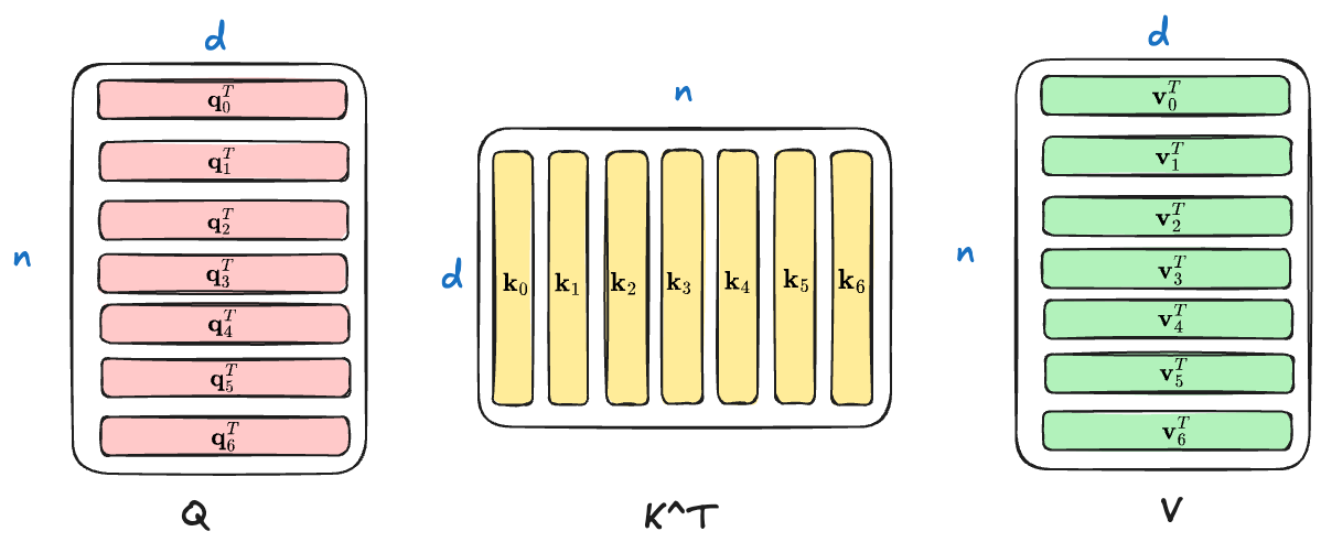
First, we need to understand how to obtain $\mathbf Q,\mathbf K,\mathbf V$ matrices. Let $\mathbf x_{1:n}$ represent the vector represent of the $n$ input tokens. By applying weighted transformation with the matrices $\mathbf W^Q, \mathbf W^K, \mathbf W^V$ (essentially matrix multiplication) we obtain $\mathbf Q,\mathbf K, \mathbf V$.

$$ \mathbf Q,\mathbf K,\mathbf V\in\mathcal{R}^{n\times d} $$

I use the Exclidraw to draw a diagram to help you understand the shape of $\mathbf Q,\mathbf K,\mathbf V$.

And then let’s see the core part of the self-attention mechanism:

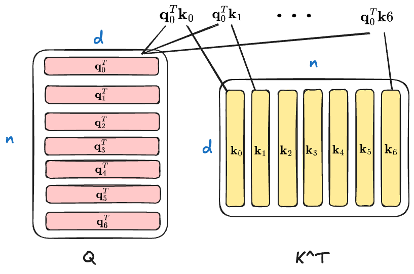
$$ \mathbf Q\mathbf K^T\in\mathcal R^{n\times n} $$

The $\mathbf Q\mathbf K^T$ would yield a matrix with $n\times n$ (the $n$ is the input length) shape, where each position $(i, j)$ represent the inner product (that is, $\mathbf q_i^T\mathbf k_j$) of $\mathbf q_i$ and $\mathbf k_j$. Therefore, the $\mathbf Q\mathbf K^T$ is a token-to-token attention score matrix. Let’s take $\mathbf q_0$ for an example.

Now, apply the $\texttt{softmax}$ on the attention score matrix for normalization, ensuring that the sum of attention score in each rowof the attention score matrix is 1.

$$ \texttt{softmax}(\mathbf Q\mathbf K^T)\in\mathcal R^{n\times n} $$

Finally, multiply the normalized attention score matrix with the value matrix $\mathbf V$

$$ \texttt{softmax}(\mathbf Q\mathbf K^T)\mathbf V\in\mathcal R^{n\times d} $$

This is the weighted sum mentioned earlier. For example, if we consider token $0$, its attention score with all token $j$ is

$$ [\mathbf q_0^T\mathbf k_0, \mathbf q_0^T\mathbf k_1, \mathbf q_0^T\mathbf k_2, …, \mathbf q_0^T\mathbf k_j]=[a_{00}, a_{01}, …,a_{0j}] $$

The weighted sum for token $0$ can be formulated as the following equation.

$$ \sum_j(\mathbf q_0^T\mathbf k_j)\mathbf v_j=\sum_j a_{0j}\mathbf v_j $$

The following diagram may help you catch this idea.

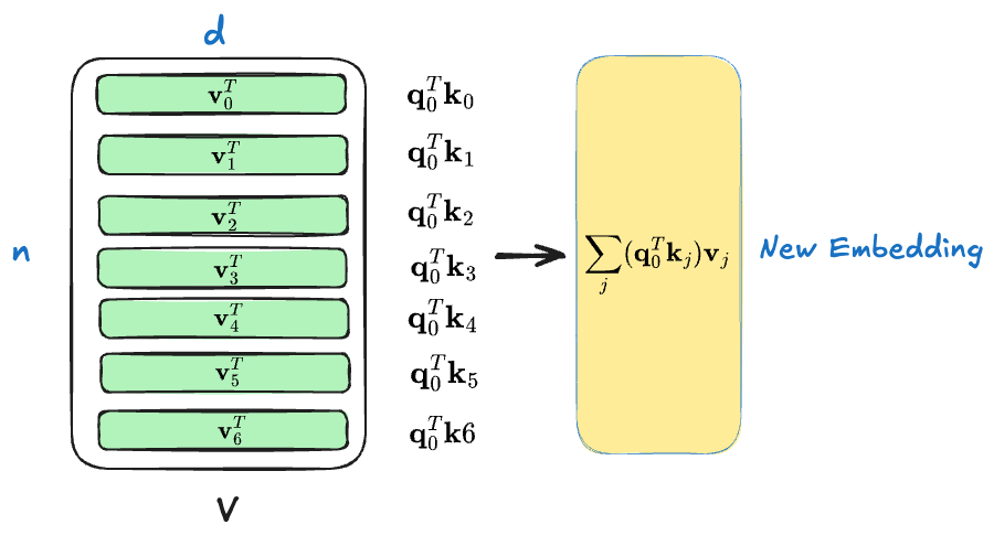
That is the final new embedding for the token $0$, and all other tokens follow the same manner to get updates.

You may notice that I didn’t explain the $\sqrt{d}$ in the denominator, what’s the purpose? In the original paper¹, the authors suspect that for large values of $d$, the dot products grow large in magnitude, pushing the softmax function into regions where it has extremely small gradients.

The $\sqrt d$ is the L2 norm of a vector with length $d$. For example, the vector $[1, 1]$’s length is 2 and its L2 norm is $\sqrt d$.

The implementation

Now, let’s try to implement the naive attention from scratch. There are some to be noticed:

• We don’t need to use 3 nn.Linear to get $\mathbf W^K, \mathbf W^Q, \mathbf W^V$. A better solution is changing the out_features and split the output into $\mathbf Q, \mathbf K, \mathbf V$
• The unidirectional self-attention can be implemented using the masking trick, that is, we mask all positions (assign them with -float('inf')) which does need to do self-attention computation (the upper triangular).

The implementation of naive self-attention is presented below, with additional comments for clarity.

import math
import torch
import torch.nn as nn
import torch.nn.functional as F

class NaiveAttention(nn.Module):
    def __init__(self, n_embd: int, block_size: int):
        super().__init__()
        self.attn = nn.Linear(n_embd, 3 * n_embd)
        self.n_embd = n_embd
        self.register_buffer(
            "bias",
            torch.tril(torch.ones(block_size, block_size)).view(
                1,
                block_size,
                block_size,
            ),
        )

    def forward(self, x):
        B, T, C = x.size()  # (batch_size, seq_len, n_embd)
        qkv = self.attn(x)  # qkv: (batch_size, seq_len, 3 * n_embd)
        q, k, v = qkv.split(self.n_embd, dim=2)  # split in n_embd dimension
        attn = (q @ k.transpose(1, 2)) * (
            1.0 / math.sqrt(k.size(-1))
        )  # attn: (batch_size, seq_len, seq_len)
        attn = attn.masked_fill(self.bias[:, :T, :T] == 0, -float("inf"))
        attn = F.softmax(attn, dim=-1)
        # print(f"{attn=}")
        out = attn @ v  # (batch_size, seq_len, n_embd)

        return out

To check if this implementation works, we can manually create an input.

module = NaiveAttention(n_embd=4, block_size=5)
sample_input = torch.randn(1, 5, 4)

Let’s check the attention matrix (atten) and final output (out).

# attn matrix:
[[[1.0000, 0.0000, 0.0000, 0.0000, 0.0000],
  [0.3017, 0.6983, 0.0000, 0.0000, 0.0000],
  [0.3125, 0.2572, 0.4303, 0.0000, 0.0000],
  [0.2190, 0.3706, 0.2354, 0.1750, 0.0000],
  [0.1901, 0.2321, 0.1831, 0.1889, 0.2058]]]

# output:
[[[0.2348, 0.0224, 0.5836, 0.1414],
  [0.1057, 0.2104, 0.6170, 0.5556],
  [0.4593, 0.0303, 0.7982, 0.0422],
  [0.2862, 0.1033, 0.6313, 0.2689],
  [0.3003, 0.1009, 0.6536, 0.2153]]]

Wrap-up

That’s all for this post! The post aims to give you a basic understanding of how self-attention works. Therefore, I didn’t talk about more complex variants like Multi-Head Attention (MHA), Multi-Head Latent Attention(MLA), etc. I plan to write more posts about the self-attention mechanism in the future. :)

Ref