How to understand the backpropagation algorithm
Update: Backpropagation in matrix form could be found here
Intro
In the field of deep learning, optimizing the network involves a crucial process of continuously updating the weights and bias items. This is achieved by implementing the gradient descent method, which progressively minimizes the loss function. At the heart of this process lies the backpropagation algorithm, which facilitates efficient computation of gradients across the network
To better understand this concept, let us recall the formula for gradient descent. In this formula, we utilize the symbol $\theta$ to represent all the learnable parameters of the model, $J$ to represent the cost or loss function, and $\alpha$ to denote the learning rate. Thus, we can express the updating process as:
$$ \theta \leftarrow \theta - \alpha * \frac{\partial J}{\partial \theta} $$
To optimize the model continuously, it’s crucial to calculate the gradient $\frac{\partial J}{\partial \theta}$ accurately and efficiently through backpropagation. This process involves computing the partial derivatives of the loss function with respect to the model’s parameters, which are also referred to as weights and biases.
📒 Throughout the post, the terms “parameters” and “weights and biases” will be used interchangeably as they both represent the learnable elements of the model
📒 It is assumed that the reader has a basic understanding of the chain rule of derivation in mathematics to follow the explanations provided🫡
Define a model
Before we proceed, we need to define a model for subsequent derivation. For this purpose, let’s consider a simple yet classical three-layer fully connected neural network:
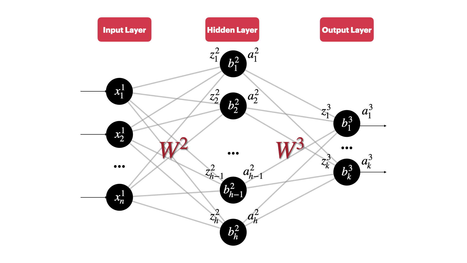
📒 Note: Uppercase letters represent matrices, and lowercase letters represent vectors (without subscripts) or scalars (with subscripts)
where:
- The network consists of an input layer with $n$ neurons, a hidden layer with $h$ neurons, and an output layer with $k$ neurons
- $x^1_j$ represents the $j$-th feature value of the input vector. Note that we start counting from 1, the output layer is the 1st layer
- $y_j$ represents the true value of the $j$-th output of the corresponding output layer
- $w^l_{jk}$ represents the weight corresponding to the link between the $k$-th neuron of the $l-1$ layer and the $j$-th neuron of the $l$ layer, Note the order of subscripts. Based on this, we can deduce that the dimensionality of $W^2$ and $W^3$ are as follows:
- $W^2\in \mathcal{R}^{h\times n}$
- $W^3\in \mathcal{R}^{k\times h}$
- $b_j^l$ represents the bias term of the $j$-th neuron of the layer $l$
- $z_j^l$ represents the weighted output of the $j$ neuron of the layer $l$
- $a_j^l$ represents the output after the activation function of the $j$-th neuron in the layer $l$
With these terms defined, we can formulate the process of forward propagation in a neural network as follows:
$$ z_j^2 = \sum_kw_{jk}^2x^1_k+b_j^2 $$
$$ a_j^2=\sigma(z_j^2) $$
$$ z_j^3 = \sum_kw_{jk}^3a_k^2+b_j^3 $$
$$ a_j^3=\sigma(z_j^3) $$
Let’s generalize $z_j^l$ and $a_j^l$:
$$ z_j^l=\sum_kw_{jk}^la^{l-1}_k+b_j^l $$
$$ a_j^l=\sigma(z_j^l) $$
The above two formulas are very important, they will be very useful in the derivation of the four formulas of backpropagation
Here we consider using the mean squared error (MSE) as the cost or loss function $J$ and the $sigmoid$ function as the activation function. Of course, the derivation process is similar if we use different cost/loss function and activation function
$$ J = \frac{1}{2k}\sum_{j=1}^k(a_j^L-y_j)^2 $$
The intuition of backpropagation
Understanding a concept at a high level before delving into its details is always beneficial. In the context of deep learning, the goal of the training process is to minimize the error between the predicted value $a^L_j$ and the actual label $y_j$ for each sample. By calculating this error, we can determine whether to increase or decrease $a^L_j$ to improve the model’s predictions. However, we can only adjust $a^L_j$ by modifying the weights $w^L_{jk}$ between the $L-1$ layer and the output layer, the bias term $b_j^L$, or the output value $a^{L-1}_k$ after the activation function in the $L-1$ layer. It’s worth mentioning that we can’t directly modify $a_k^{L-1}$, which is determined by the values of the previous weight and bias items. When we decide how to modify each weight and bias of the model backwardly based on the prediction error, we are doing backpropagation1
The above process describes how $a_j^L$ wants to adjust the weights and biases of the entire model. However, we need to consider the opinions of all neurons in the output layer, as each neuron may has a different idea of how the weights and biases should change. Ultimately, we need to update the model’s weights and biases by incorporating the opinions of all neurons in the output layer.
The four formulas of the backpropagation
The core of the backpropagation algorithm contains 4 formulas
Formula 1
$$ \delta_j^L=\frac{\partial J}{\partial a_j^L}\sigma’(z_j^L) $$
Where $L$ is the number of layers of the model($L=3$ in this example), $\delta_j^L$ represents the gradient of the $j$-th neuron in the $L$ layer
By the way, the above formula can be rewritten as $\delta^L=\nabla J\odot \sigma’(z^L)$ in vectorized form. The $\odot$ represents the element-wise multiplication
📒 Formula 1 calculates the gradient of each neuron in the output layer
How to derive this⬇️ $$ \begin{aligned} \delta_j^L&=\frac{\partial J}{\partial z_j^L} \\\ &=\sum_k\frac{\partial J}{\partial a_k^L}\frac{\partial a_k^L}{\partial z_j^L} \\\ &=\frac{\partial J}{\partial a_j^L}\frac{\partial a_j^L}{\partial z_j^L}\ (only\ \frac{\partial a_j^L}{\partial z_j^L}\ne 0) \\\ &=\frac{\partial J}{\partial a_j^L}\frac{\partial \sigma(z_j^L)}{\partial z_j^L}\ \\\ &=\frac{\partial J}{\partial a_j^L}\sigma’(z_j^L) \end{aligned} $$
Formula 2
$$ \delta^l=((w^{l+1})^T\delta^{l+1})\odot \sigma’(z^l) $$
📒 Formula 2 calculates the gradient vector of any layer $l$. It is worth noting how this formula links the gradient of layer $l$ with that of layer $l+1$. This allows us to compute the gradient of a previous layer using the gradients of subsequent layers
How to derive this⬇️ $$ \begin{aligned} \delta_j^l&=\frac{\partial J}{\partial z_j^l} \\\ &=\sum_k\frac{\partial J}{\partial z_k^{l+1}}\frac{\partial z_k^{l+1}}{\partial z_j^l} \\\ &=\sum_k\delta_k^{l+1}\frac{\partial }{\partial z_j^l}z_k^{l+1} \end{aligned} $$
Note that $\frac{\partial }{\partial z_j^l}z_k^{l+1} = \frac{\partial }{\partial z_j^l}\ \sum_pw^{l+1}_{kp}\sigma(z_p^l)+b^{l+1}_k$
The derivative only exists when $p=j$, so the solution to the above formula is $w^{l+1}_{kj}\sigma’(z_j^l)$.
That is, we have shown that $\delta_j^l=\sum_k\delta_k^{l+1}\ w^{l+1}_{kj}\sigma’(z_j^l)$
$\sum_k\delta_k^{l+1}w^{l+1}_{kj}$ is actually calculating the inner product of 2 vectors, so it can be rewritten as a vectorized form - $\delta^l=((w^{l+1})^T\delta^{l+1})\odot \sigma’(z^l)$
Formula 3
$$ \frac{\partial J}{\partial b^l_j}=\delta_j^l $$
📒 Formula 3 can be used to calculate the gradient of any bias term in the model
How to derive this⬇️ $$ \begin{aligned} \frac{\partial J}{\partial b^l_j}&= \frac{\partial J}{\partial z^l_j}\frac{\partial z^l_j}{\partial b^l_j} \\\ &= \delta_j^l \frac{\partial}{\partial b^l_j}\sum_kw^l_{jk}a^{l-1}_j+b^l_j\\\ &= \delta_j^l \end{aligned} $$
Note that the first equal sign above is similar to the derivation of formula 1. I skipped the process of removing $\sum_k$
Formula 4
$$ \frac{\partial J}{\partial w_{jk}^l}=a_k^{l-1}\delta_j^l $$
📒 Formula 4 can be used to calculate the gradient of any weight term in the model
How to derive this⬇️ $$ \begin{aligned} \frac{\partial J}{\partial w_{jk}^l}&=\frac{\partial J}{\partial z^l_j}\frac{\partial z^l_j}{\partial w_{jk}^l} \\\ &=\frac{\partial J}{\partial z^l_j}\frac{\partial }{\partial w_{jk}^l}\sum_pw_{jp}^la_p^{l-1}+b_j^l \\\ &=\delta_j^l\frac{\partial }{\partial w_{jk}^l}\sum_kw_{jk}^la_k^{l-1}+b_j^l \\\ &=\delta_j^la_k^{l-1} \end{aligned} $$
Backpropagation algorithm procedure
Based on the aforementioned formulas, we can know the whole process of backpropagation will be:
- Forward propagation, compute $z_j^l$,$a_j^l$ for each neuron in each layer
- Compute $\delta^L$ in the output layer based on the formula 1
- Repeat the following process backwardly
- Calculate the gradient vector $\delta^l$ for each layer based on formula2. Note that we can always compute $\delta^l$ using $\delta^{l+1}$ :)
- Calculate the gradient of each bias term $b^l_j$ based on formula 3, which is equal to $\delta^l_j$
- Calculate the gradient of each weight $w^l_{jk}$ based on formula 4, which is equal to $\delta_j^la_k^{l-1}$
The above process also answers the question of why backpropagation is an efficient algorithm:
- 👍 When calculating the gradient vector $\delta^l$ for the $l$-th layer based on formula 2, $\delta^{l+1}$ has already been computed and there is no need to start from scratch at the output layer.
- 👍 By directly calculating the gradient of the loss function with respect to the current layer’s weights and bias terms using formulas 3 and 4, we avoid computing intermediate gradient results.
Wrap up
The above is the entire process of the backpropagation algorithm. Although it involves a lot of formulas and notation, it is still relatively easy to understand. When reviewing the backpropagation algorithm, I found some points that may help readers understand it:
- Backpropagation is an algorithm for a single sample, so when you derive the formulas, you only need to consider one sample as the input of the model
- When deriving the formulas, start from the scalar form and then generalize it into vectorized form. Don’t start with vectorized form or you may get stuck easily.
Of course, if you’ve solid basics of math, ignore what I just said
That’s all, thanks for reading👋