Demystifying Pytorch's Strides Format
Intro
Even though I have been using Numpy and Pytorch for a long time, I never really knew how they implemented the underlying tensors and why they are so efficient. Recently, while studying the course Deep Learning Systems, I finally got the opportunity to try implementing tensors on my own. After going through the process, my understanding of tensors is much better 🧐
As a Pytorch user, is it necessary to understand the underlying tensor storage mechanism? I believe it is essential. In most cases, understanding the underlying principles helps you grasp higher-level concepts better. For example, understanding the tensor storage mechanism can help you answer the following questions:
- Does broadcasting involve copying arrays?
- What does
contiguousdo in Pytorch, and why is this function needed?
Row-major and column-major
Let’s start with a simple 2D array, A 2D array occupies a contiguous location in memory, but how it is stored, whether using row-major or column-major, may vary.
Let’s say we have a 2D array A whose size is $2\times 3$
[[0.2949, 0.9608, 0.0965],
 [0.5463, 0.4176, 0.8146]]
If we use row-major, then the memory layout(denoted as A_in_row) would be:
[0.2949, 0.9608, 0.0965, 0.5463, 0.4176, 0.8146]To access (i, j) when using row-major, the equations says:
A[i][j] = A_in_row[i * A.shape[1] + j]If we use column-major, then the memory layout(denoted as A_in_col) would be:
[0.2949, 0.5463, 0.9608, 0.4176, 0.0965, 0.8146]To access (i, j) when using column-major, the equations says:
A[i][j] = A_in_col[j * A.shape[0] + i]Strides format
Note: I will use continuous/contiguous/compact interchangeably.
At the low level, tensors can be stored either by rows or columns. Both Numpy and PyTorch adopt the approach of storing tensors by rows. Regardless of the tensor’s dimension, the underlying storage always occupies continuous memory space. Now, the question arises: How do we access the data at the desired positions?
The answer is strides format. We may regard the strides format as a generalization version of the two previous indexing formats. Let’s consider a tensor of $N$ dimensions(0-based), and its underlying storage is represented as A_internal. If we want to access A[i0][i1][i2]..., the indexing is done as follows:
A[i0][i1][i2]... = A_internal[
    stride_offset
    + i0 * A.strides[0]
    + i1 * A.strides[1]
    + i2 * A.strides[2]
    + ...
    + in-1 * A.strides[n-1]
]
The strides format has two components:
offset- the offset of the tensor relative to the underlying storagestridesarray, whose length is equal to the number of dimensions of the tensor.strides[i]indicates how many “elements” need to be skipped in memory to move “one unit” in the $i$-th dimension of the tensor
For example, considering the earlier example of a 2D array, if we interpret it using the strides format
A[i][j] = A_in_row[
0
+ i * A.shape[1]
+ j * 1
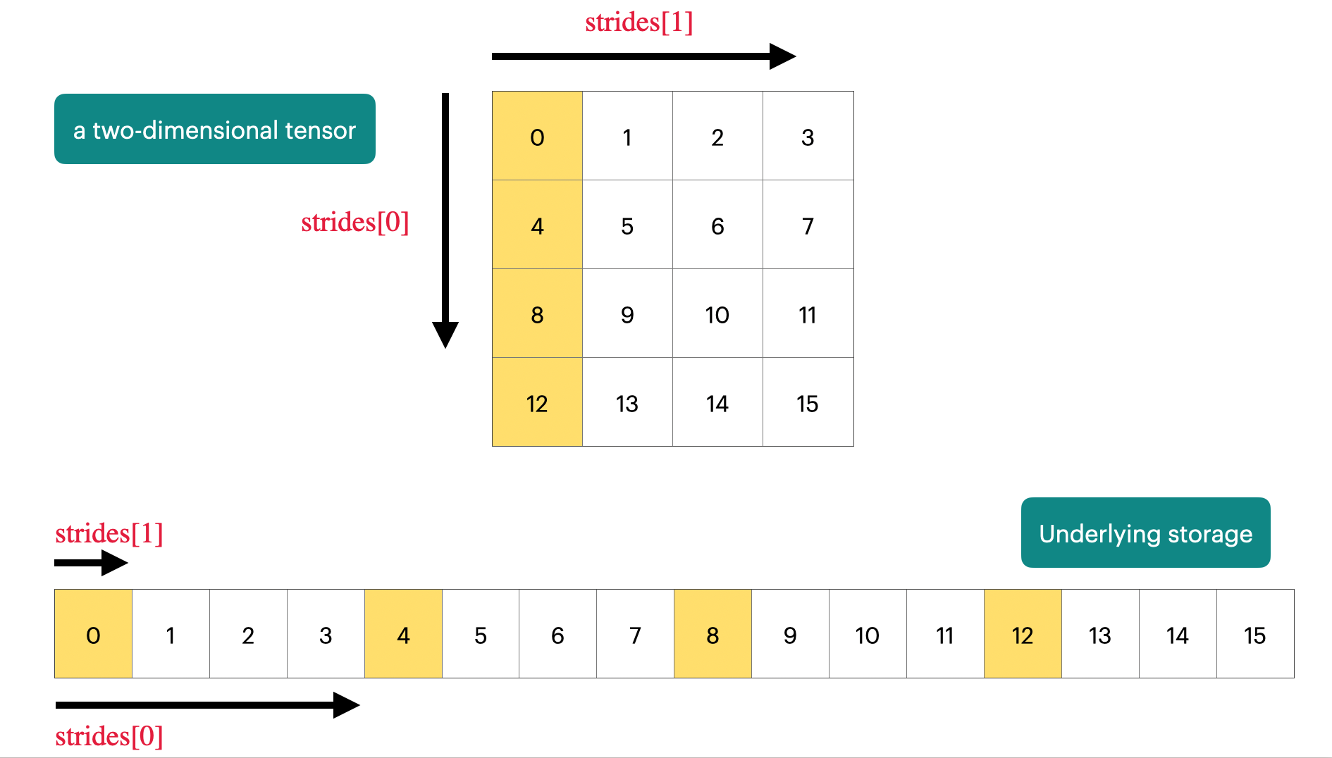
]For a 2D array of size (A.shape[0], A.shape[1]), its offset is 0, and the strides array is [A.shape[1], 1](row-major). 🤔️ This means that moving “one unit” in the first dimension requires skipping A.shape[1] elements in the underlying memory, where A.shape[1] is the length of each row
I made this image to give you better intuition :)
🧐 How to obtain the strides array for an $N$ dimensional tensor? Let’s say we want to calculate strides[k] for the $k$-th dimension. We know the semantic of strides[k] is the elements to skip in the underlying memory to moving “one unit” in the $k$-th dimension, If the memory layout of the tensor is continuous, then the answer would be the product of $k+1,k+2,…, N-1$. If $k=N-1$, then strides[N - 1] = 1
The mathematical formula is as follows: $$strides[k]=\prod_{i=k+1}^{N-1}shape[i]$$
💡 It is important to reiterate that the above formula holds only when the tensor’s underlying memory layout is contiguous.
Why strides?
After understanding the strides format. The next question would be: Why do we need the strides format and what benefits it brings? The most significant advantage is that many tensor operations can be performed in a zero-copy manner. By using the strides format, the concepts of “underlying storage” and “views” are separated. Now let’s talk about some common tensor operations
print_internal function
Before we start to investigate the tensor operations, we need to write a helper function such that we can get the underlying storage.
Pytorch provides us with the data_ptr API, which will return the address of the first element of a tensor.
Then, by using the storage().nbytes() method provided by PyTorch, we can determine the amount of memory space the tensor’s underlying storage occupies(in bytes)1. Additionally, the dtype attribute of the tensor informs us about the size of each element. For example, torch.float32 occupies 4 bytes
Finally, we can use the ctypes.string_at(address, size=-1) function to read the tensor as a C-style string (buffer), and torch.frombuffer can be used to create a tensor from this buffer.
Putting it all together, we can write this helper function called print_internal:
def print_internal(t: torch.Tensor):
    print(
        torch.frombuffer(
            ctypes.string_at(t.data_ptr(), t.storage().nbytes()), dtype=t.dtype
        )
    )
Now we create a tensor t with dimension (1, 2, 3, 4) and observe its underlying representation. The subsequent operations and explanations will be based on this tensor t
torch.arange(0, 24).reshape(1, 2, 3, 4)
print(t)
# tensor([[[[ 0,  1,  2,  3],
#           [ 4,  5,  6,  7],
#           [ 8,  9, 10, 11]],

#          [[12, 13, 14, 15],
#           [16, 17, 18, 19],
#           [20, 21, 22, 23]]]])

print(t.stride())
# (24, 12, 4, 1)

print_internal(t)
# tensor([0,  1,  2,  3,
#         4,  5,  6,  7,
#         8,  9, 10, 11,
#         12, 13, 14, 15,
#         16, 17, 18, 19,
#         20, 21, 22, 23])
By using the formula we previously talked about, we know the strides of t should be (2 * 3 * 4, 3 * 4, 4, 1), that is, (24, 12, 4, 1). The t.stride() will give us the strides array maintained by Pytorch. Indeed, it gives us the answer which is exactly what we expected.
permute operations
Suppose we rearrange the dimensions with permute, how does strides change?
print(t.stride())
# (24, 12, 4, 1)

print(t.permute((1, 2, 3, 0)).is_contiguous())
# True

print(t.permute((1, 2, 3, 0)).stride())
# (12, 4, 1, 24)

print(t.permute((0, 2, 3, 1)).is_contiguous())
# False

print(t.permute((0, 2, 3, 1)).stride())
# (24, 4, 1, 12)

print(t.permute((1, 0, 3, 2)).is_contiguous())
# False

print(t.permute((1, 0, 3, 2)).stride())
# (12, 24, 1, 4)

print_internal(t.permute((1, 2, 3, 0)))
# tensor([0,  1,  2,  3,
#         4,  5,  6,  7,
#         8,  9, 10, 11,
#         12, 13, 14, 15,
#         16, 17, 18, 19,
#         20, 21, 22, 23])
As indicated by these examples, the permute operation will not change offset. However, the permute operation will usually make the underlying storage incompact. Although we can use the new_shape after permuting to re-calculate the strides array, a better way would be just permute the original strides array. The output of print_internal indicates that the permute operation is lazy2.
broadcast_to operation
Broadcast_to operation is an interesting operation. Before knowing the internals, you might think that broadcasting involves copying along the corresponding dimensions. However, there is no copying under the hood. Pytorch just change the strides array. More specifically, Pytorch will set stride[k] = 0 if its size is one before broadcasting3.
Let’s try to do broadcasting along the first dimension of tensor t and observe how the shape and strides will change
print(t.broadcast_to((2, 2, 3, 4)).is_contiguous())
# False

print(t.broadcast_to((2, 2, 3, 4)).shape)
# torch.Size([2, 2, 3, 4])

print(t.stride())
# (24, 12, 4, 1)

print(t.broadcast_to((2, 2, 3, 4)).stride())
# (0, 12, 4, 1)

print_internal(t.broadcast_to((2, 2, 3, 4)))
# tensor([0,  1,  2,  3,
#         4,  5,  6,  7,
#         8,  9, 10, 11,
#         12, 13, 14, 15,
#         16, 17, 18, 19,
#         20, 21, 22, 23])
Surprisingly, Pytorch does not allocate memory, and copy elements in the dimension got broadcasted. The only thing that changed is the strides array. Pause for a second and try to figure out what’s the meaning of setting stride as 0. It means we don’t need to skip any elements along this dimension, which indicates we are referring to the same data(same memory location).
reshape operation and contiguous operation
The indexing operation may modify the offset because the resulting tensor after indexing may not start from the first element of the original underlying storage. Moreover, the indexing operation may access the non-contiguous parts of the underlying storage. So the indexing operation will help us to understand the reshape and contiguous operations better.
Let’s say we want to get the following tensor from t
[[[2,
   6,
   10],
  [14,
   18,
   22]]]
The corresponding indexing operation is
print(t[:, :, :, 2])
# tensor([[[ 2,  6, 10],
#          [14, 18, 22]]])
Note that this operation aligns with what I mentioned earlier:
- the
offsetwill change because the resulting tensor starts from2rather than0 - The elements accessed by indexing are not contiguous in the original memory
The following code proves our speculation
print(t.storage_offset())
# 0

print(t[:, :, :, 2].storage_offset())
# 2

print(t[:, :, :, 2].is_contiguous())
# False
Now let’s observe the underlying storage
print_internal(t[:, :, :, 2])
# tensor([        2,  3,
#         4,  5,  6,  7,
#         8,  9, 10, 11,
#         12, 13, 14, 15,
#         16, 17, 18, 19,
#         20, 21, 22, 23
#         1152921504606846976, -8070441752123218147]])
# ignore the last row because t.data_ptr() has changed but t.storage().nbytes()
# kept the same.
# As a result, we read 2 invalid elements and get 2 meaningless values
Pytorch’s tensor has a method called storage_offset() which shows the offset in the underlying storage. As we can see, now it starts from the second position in the underlying storage, which corresponds to the first element 2 of t[:, :, :, 2]. And the underlying storage is still the same
Note: Because the underlying storage remains unchanged,
t.storage().nbytes()remains the same. Thedata_ptr()will give us the address of the second element. As a result, the printed underlying array will have two additional meaningless positions (as seen in the last row), resulting in two extra irrelevant numbers.
🤔️ Let’s try to use reshape(3, 2) after indexing and observe the underlying storage
print_internal(t[:, :, :, 2].reshape(3, 2))
# tensor([        2,  3,
#         4,  5,  6,  7,
#         8,  9, 10, 11,
#         12, 13, 14, 15,
#         16, 17, 18, 19,
#         20, 21, 22, 23
#         1152921504606846976, -8070441752123218147]])
We find that the reshape operation does not change the underlying storage. This aligns with what the documentation states: When possible, the returned tensor will be a view of input4
What if we want the tensor after reshape to have compact storage? We can use the contiguous method
print_internal(t[:, :, :, 2].reshape(3, 2).contiguous())
# tensor([ 2,  6, 10, 14, 18, 22])
😺 By chaining reshape and contiguous operations, we make the underlying storage compact. And the strides array should align with the aforementioned formula:
# before contiguous
print(t[:, :, :, 2].reshape(3, 2).stride())
# (8, 4)

# after contiguous
print(t[:, :, :, 2].reshape(3, 2).contiguous().shape)
# (3, 2)
print(t[:, :, :, 2].reshape(3, 2).contiguous().stride())
# (2, 1)
🧐 One challenging question for you, how indexing operation will change the strides array?
Let’s use the previous indexing operation as an example. First, after indexing, the new dimensions should be (1, 2, 3). The indexing pattern [:, :, :, 2] results in a non-compact underlying storage. So we can not just compute the strides array by the rule. Therefore, we have to reason the strides array based on the definitions. Let’s assume the strides array of t[:, :, :, 2] is [x, y, z]
We can observe which elements are included in t[:, :, :, 2]
print(t[:, :, :, 2])
# tensor([[[ 2,  6, 10],
#          [14, 18, 22]]])
Because the tensor t starts from 0 and increments by one, we can just compute the strides based on the values(a little trick)
- for
z, we find2 -> 6 -> 10, that is, we skip 4 elements each time. Soz = 4 - for
y, we find2 -> 14,6 -> 18,10 -> 22, we skip 12 elements each time. Soy = 12 - for
x, since the underlying storage has not changed, the original tensorthasstrides[0] = 24. Imagining that the first dimension is not 1 but a bigger value, we would need to skipstrides[0]elements each time. Sox = 24
We claim that the strides of t[:, :, :, 2] should be (24, 12, 4)
Let’s call the API to check if our claim is correct
print(t.stride())
# (24, 12, 4, 1)

print(t[:, :, :, 2].stride())
# (24, 12, 4)

# what if the first dimension is not 1 but 2?
another_t = torch.arange(0, 48).reshape(2, 2, 3, 4)
print(another_t[:, :, :, 2])
# tensor([[[ 2,  6, 10],
#          [14, 18, 22]],

#         [[26, 30, 34],
#          [38, 42, 46]]])

# you can see that 2 -> 26, 6 -> 30, 10 -> 35
# , so the stride[0] = 24 is true
The output meets our expectations
However, the indexing operations can be much more complex than our naive [:, :, :, 2] like [2, 1:3, 1:6:3], and in such cases, how do strides and offset change? I won’t elaborate on this, but here’s a hint: convert each format into Python’s Slice object and then reason through the definition of strides[i]
Wrap up
As you can see, many operations on Pytorch tensors are achieved by modifying the offset or(and) strides array. This approach allows many operations to maintain zero-copy overhead, leading to high efficiency. Moreover, this enables the lazy operations. Understanding the strides format helps in constructing a mental model of tensors and facilitates a better understanding of tensor operation code. I would also recommend watching the awesome video which talks about the cool tricks that manipulating strides to perform convolution efficiently
Now we can answer the questions raised earlier:
- Does broadcasting involve copying arrays?
- No, broadcasting will only change the
stridesarray
- No, broadcasting will only change the
- What does
contiguousdo in Pytorch, and why is this function needed?- By using
contiguous, we can make the underlying storage compact. Although this may involve copying, it is beneficial for later calculation because of the memory locality.
- By using