LLM inference optimization - KV Cache

Background

The secret behind LLM is that it will generate tokens one by one based on all the previous tokens.

Let’s assume that we have already generated $t$ tokens, denoted by $x_{1:t}$. In the next iteration, the LLM will generate $x_{1:t+1}$. Note that the first $t$ tokens are the same.

$$x_{1:t+1}=\text{LLM}(x_{1:t})$$

The next iteration is similar.

$$x_{1:t+2}=\text{LLM}(x_{1:t+1})$$

In summary, in each iteration, we will use the output of the previous round as a new input for the LLM. Generally, this process will continue until the output reaches the maximum length we predefined or the LLM itself generates a special token, signifying the completion of the generating process.

Demystify the KV Cache

Simply overserving two consecutive inference calculations is sufficient to understand why the redundant computations are present

For example

$$ x_{1:t+1}=\text{LLM}(x_{1:t}) $$

The input of the LLM is $x_{1:t}$. Let’s focus on the last token $x_t$, whose query vector will undergo dot product computation with the key vectors generated by each of the preceding tokens, including itself.

$$\mathbf q_{t}^T\mathbf k_{1},\mathbf q_{t}^T\mathbf k_{2},…,\mathbf q_{t}^T\mathbf k_{t}$$

The next step is

$$ x_{1:t+2}=\text{LLM}(x_{1:t+1}) $$

The input of the LLM is $x_{1:t+1}$. The last token $x_{t+1}$ will also undergo dot product computation with the key vectors generated by each of the preceding tokens, including itself.

$$\mathbf q_{t+1}^T\mathbf k_{1},\mathbf q_{t+1}^T\mathbf k_{2},…,\mathbf q_{t+1}^T\mathbf k_{t+1}$$

What about the $x_t$ token?

$$\mathbf q_{t}^T\mathbf k_{1},\mathbf q_{t}^T\mathbf k_{2},…,\mathbf q_{t}^T\mathbf k_{t}$$

We can see that the computations are redundant compared to the previous round. The same logic applies to tokens before $x_t$. We need to recalculate all the key vectors and value vectors for $x_{1:t}$, even though the values of these vectors actually remain unchanged🧐.

After applying the KV Cache, in each round except the first one, we only need to focus on the last input token. We will compute its query, key, and value vectors and use these 3 new vectors to perform a self-attention operation with all the cached key/value vectors of preceding tokens.

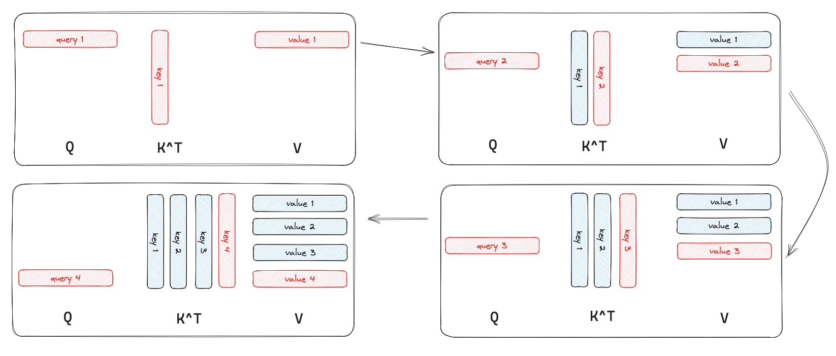
I drew a simple picture to show what happened we when used the KV Cache to speed up the inference process. Consider that the LLM generates 4 tokens starting from scratch, where the blue part represents the values that are cached, and the red part indicates what’s not cached

The performance of the KV Cache

The principle behind accelerating inference with the KV Cache is as follows: in the self-attention layer, instead of performing the matrix multiplication $\mathbf Q\mathbf K^T$ in each iteration, we only need to perform vector-matrix multiplication between the query vector $\mathbf q$ of the last token of each input and $\mathbf K$, and then we update the KV Cache.

Incorporating the KV Cache allows the inference process of LLM to be viewed as two stages

1. In the first iteration, the KV Cache is empty, so we need to compute all the key, query, and value vectors for these tokens, and we will cache the key/value vectors.
2. For every subsequent iteration, you only need to compute the key, query, and value vector for the new token and update the KV Cache.

Then, what’s the price of the KV Cache? The main cost is that it will increase the GPU peak memory usage. You can find a memory usage comparison of enabling or disabling the KV Cache here. I will put some summarization below.

• Enable the KV Cache - 2 * hidden_size * num_layers * decoder_length
  • 2: because we need to cache the key vector and value vector
  • hidden_size: the length of the key or value vector
  • num_layers: the key and value vectors need to be cached in each layer
  • decoder_length: the length of sequence length
• Disable the KV Cache - 2 * hidden_size * 1 * decoder_length

KV Cache API

Huggingface provides an API called model.generate. It has a parameter called use_cache, which is set to True by default¹.

Ref