Reading Notes: Outrageously Large Neural Networks-The Sparsely-Gated Mixture-of-Experts Layer

Motivations

The model’s performance is related to the model’s parameter. The bigger the model is, the more performant it will be. However, the computational cost also increases. To mitigate this problem, various forms of conditional computation have been proposed to increase model performance without a proportional increase in computational costs¹.

Today I would like to share the Sparsely-Gated Mixture-of-Experts Layer (MoE) as proposed in this paper.¹

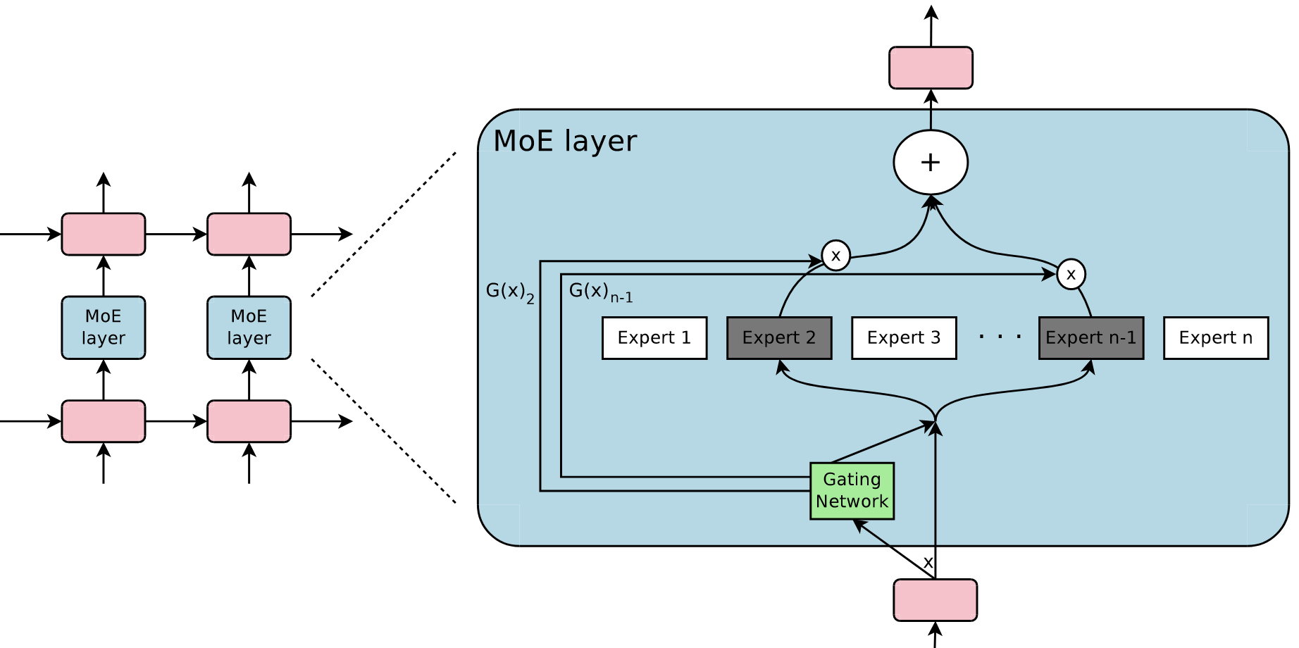
MoE architecture

There are $n$ experts in the MoE layer (denoted as $E_1, E_2, …, E_n$) and they are controlled by a gating network $G$. The output of the gating network $G$ is a vector with length $n$.

Let’s use $x$ to represent the input, $G(x)$ to represent the output of the gating network $G$, and $E_i(x)$ to represent the output of expert $E_i$. Then the output of the MoE layer (denoted as $y$) is

$$ y=\sum_{i=1}^nG(x)_iE_i(x) $$

Note the subscript $i$ in $G(x)_i$, which represents the $i$-th position of $G(x)$. From this equation, we know that the output of the MoE layer is the weighted sum of experts’ output.

If the $G(x)_i =0$ is satisfied, then the corresponding $E_i(x)$ does not need to be calculated, which would decrease the computational cost. If there exist many positions where $G(x)_i=0$, that is, the output of gating network $G$ is sparse, the computational cost should be very low.

Expert

An expert is a trainable network. In this paper, the authors just use a simple FFN layer.

Gating Network

A naive idea is multiple the input $x$ with the weight matrix $W_g$, and then apply the $\texttt{Softmax}$ function on it (note that the output of $\texttt{Softmax}$ is a probability distribution whose summation is 1)

$$ \texttt{Softmax}(x\cdot W_g) $$

However, it is not sparse. So the authors add the following components

1. Add the tunable Gaussian noise to $x\cdot W_g$
2. Keep the top k values, and set the rest to $-\infty$ (which causes the corresponding gate values to 0 after $\texttt{Softmax}$)

What is the tunable Gaussian? The authors multiply the Gaussian noise by the Softplus function while setting the input of Softplus as $x\cdot W_{noise}$. The weight matrix $W_{noise}$ also plays a regulatory role. In this way, the Gaussian noise can be independently controlled in each different MoE layer.

Let’s translate the text description to the following equations.

$$ \begin{split} G(x)&=\texttt{Softmax}(KeepTopK(H(x), k)) \\\ H(x)_i&=(x\cdot W_g)_i + \texttt{StandardNormal}()\cdot\texttt{Softplus}\big((x\cdot W_{noise})_i\big) \\\ KeepTopK(v,k)_i&= \begin{cases} v_i & \texttt{if }v_i\texttt{ is in the top }k\texttt{ elements of } v\\\ -\infty & \texttt{otherwise} \end{cases} \end{split} $$

MoE optimizations

Batch size

Increasing the batch size improves the computational efficiency. In the MoE architecture, assuming the batch size is $b$, in each iteration, $k$ experts are activated out of $n$. Then we know that the equivalent batch size is

$$ \frac{kb}{n} $$

However, we can not just keep increasing the batch size $b$ because the GPU memory is limited. To solve this problem, the authors suggest using data parallelism but keeping only one copy of each export. As for the standard layers and the gating networks, they will be duplicated in different devices. Each expert in the MoE layer would receive a combined batch consisting of the relevant examples from all of the data-parallel input batches¹. If there are $d$ devices and each one process a batch of size $b$, then the equivalent batch size is

$$ \frac{kbd}{n} $$

So we can get more devices to increase the batch size.

Balancing expert utilizations

In the course of experiments, the authors observed that the gating network $G$ would always choose a few experts after converging. This phenomenon would be self-reinforcing as the favored experts are trained more rapidly and thus are selected even more by the gating network $G$¹.

To mitigate this problem, the authors proposed a soft constraint approach: define the importance of an expert. Let’s say now we have a batch of data (denoted as $X$) and for expert $E_i$, the importance of $E_i$ is $\sum_{x\in X} G(x)_i$. Thus, all the experts’ importances can be represented as $Importance(X)$:

$$ Importance(X)=\sum_{x\in X}G(x) $$

Note that $Importance(X)$ is a vector with length $n$, and each position is the corresponding importance of the specific expert. With the $Importance(X)$ we can define an additional loss

$$ L_{importance}(X)=w_{importance}\cdot\texttt{CV}(Importance(X))^2 $$

This loss term would be added to the overall loss function. The $w_{importance}$ is a hyper-parameter and the $\texttt{CV}$ is the coefficient of variation. The $\texttt{CV}$ is a measurement of dispersion. We can imagine that if the importance of experts are varied, the dispersion would be higher and cause the loss $L_{importance}(X)$ higher. So this additional loss has the effect that encouraging all experts to have equal importance

Experiments result

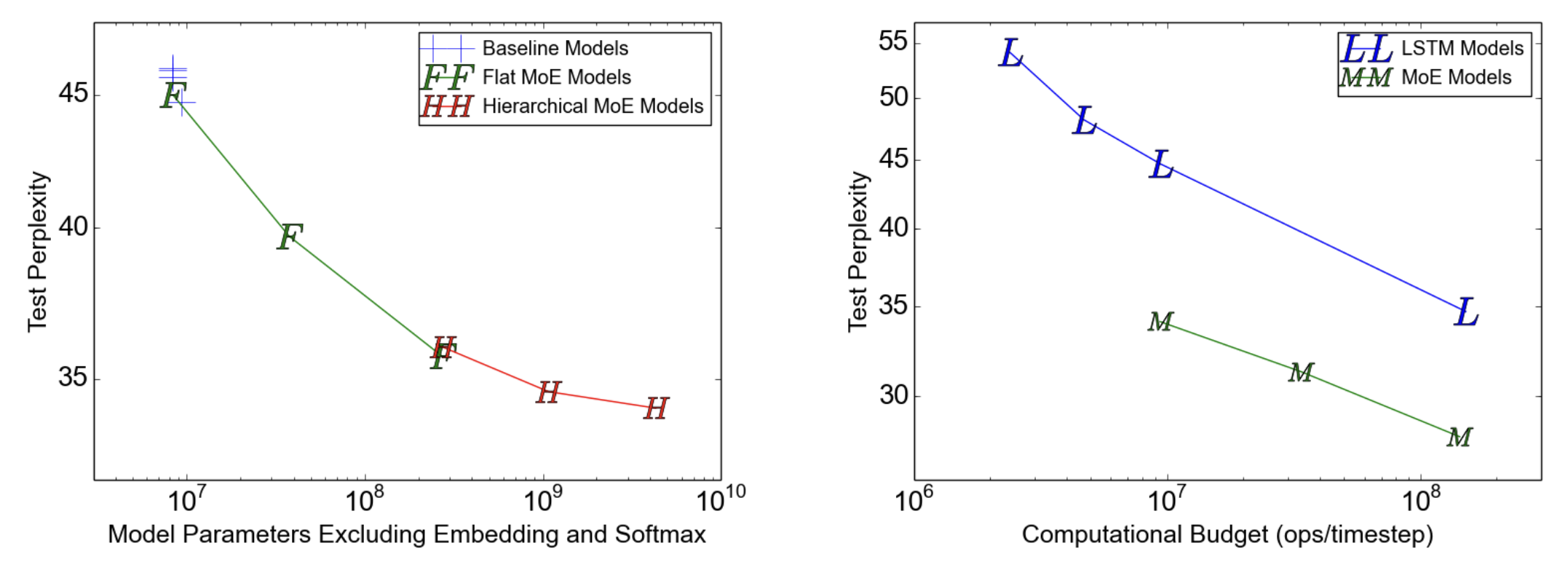
The two diagrams demonstrated the following conclusions:

1. All MoE models (flat or hierarchical) perform better than the baseline model.
2. Hierarchical MoE is slightly better than the flat MoE.
3. The MoE model performs better when the computational cost is fixed (the y-axis).

Wrap-up

To summarize, the MoE architecture enables us to increase the model parameters without a proportional increase in computational cost. In the model inference phase, only k experts would be activated, which decreases the inference cost. However, all the weight and bias of the model should be loaded into the GPU memory. 🤔

Refs