Time-series data downsampling: LTTB & MinMaxLTTB

Background

Recently, I needed to process some time-series data at work and perform downsampling. To do this, I dug into the LTTB (Largest-Triangle-Three-Buckets) and MinMaxLTTB algorithms.

Technically speaking, time-series downsampling generally falls into two categories¹:

• Characteristic Preserving: The goal is to keep statistical properties (like mean, variance, etc.) as consistent as possible before and after downsampling.
• Value Preserving: This approach selects representative data points directly from the raw dataset to preserve the overall visual shape.

Both LTTB and MinMaxLTTB are essentially value-preserving algorithms—their core objective is to retain the original trend and shape of the data after downsampling.

LTTB algorithm

The name LTTB stands for Largest-Triangle-Three-Buckets, which breaks down pretty intuitively:

• Largest Triangle: LTTB selects downsampled points by maximizing the area of the triangles formed between them.
• Three Buckets: The algorithm divides the entire dataset into multiple buckets, analyzing three adjacent buckets at a time to form a triangle by picking one point from each.

Looking at the high-level summary, a few questions come to mind:

1. How is the dataset split into buckets, and what is the criterion?
2. How is a point selected from each bucket? Do all three buckets follow the same selection strategy?
3. Why does maximizing triangle area translate to retaining the original shape?

In my opinion, the third question is the most fascinating part of the algorithm, but it’s tough to explain without a solid understanding of how LTTB actually works. Questions 1 and 2, on the other hand, cover the implementation details.

So, let’s first walk through how the LTTB algorithm works step-by-step, and then tackle these questions head-on.

Input:

• $N$ data points denotes as $p_1, p_2, \ldots, p_N$ (each node has $x$ and $y$).
• $M$ ($2 < M < N$), the target nodes count after downsampling.

Output: $M$ data pointss. Note that the $p_1$ and $p_N$ are always included

Algorithm:

1. Edge case handling: if $M \ge N$, this algorithm returns the origin $N$ data points directly. If $M \le 2$, return ${p_1, p_N}$
2. Pick $p_1$
3. Divide the middle $N - 2$ data points into $M - 2$ buckets, each of size $B = \frac{N - 2}{M - 2}$
4. Process each bucket $i = 0, 1, \ldots, M-3$ sequentially:
   • Calculate the average point $\bar{p} = (\bar{x}, \bar{y})$ across all data points in the next bucket $i+1$
   • Let $a$ be the point selected from the previous step (initialized to $p_1$)
   • Iterate over every data point $p_j$ in current bucket $i$, compute the area of the triangle formed by $a, p_j, \bar{p}$ using the cross-product formula $S_j = \frac{1}{2}\left|(x_a - \bar{x})(y_j - y_a) - (x_a - x_j)(\bar{y} - y_a)\right|$. Select the point $p_j$ that maximizes $S_j$ and append it to the downsampled results.
   • Set $a$ to this newly selected data point so it can serve as the anchor for processing the next bucket.
5. Pick $p_N$

Now we have clear answers to questions 1 and 2:

1. Bucket Division: Always retain the first and last points, then distribute the remaining $N−2$ data points into $M−2$ buckets.
2. Point Selection: Iterate through all available data points in the current bucket to find the one that forms the largest triangle. This calculation depends on two reference points:
   • The point selected from the previous bucket.
   • The “average point” of the next bucket. The intuition here is simple: the average point serves as an approximation of the upcoming data trend in the next bucket.

That leaves us with question 3: Why specifically choose the data point that maximizes the triangle’s area? Rather than walking through a rigorous proof, I’d like to build an intuitive mental model for this. When downsampling while preserving visual shape, the key is to retain peak/trough extreme values while stripping away minor fluctuations. If we treat the points $v_1$ and $v_3$ (see the diagram below) as fixed anchors forming the base of a triangle, the extreme point $v_2$ is typically the one with the greatest height. In other words, extreme points naturally maximize the triangle’s area.

Flipping that logic around: if our goal is to keep the overall shape intact after downsampling, maximizing triangle areas is precisely how we achieve it.

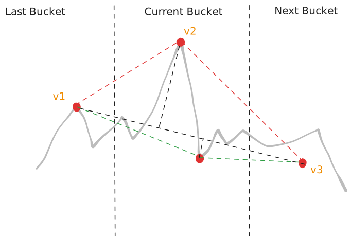
Due to its single-pass sequential processing, LTTB runs in $O(N)$ time.

Finally, let’s see how to implement it in Python.

First, we need to define a helper function that computes the area of a triangle given the three points. We also define a Point type for type annotations.

Point = tuple[int, int]

def triangle_area(p1: Point, p2: Point, p3: Point):
    return 0.5 * abs(
        (p2[0] - p1[0]) * (p3[1] - p1[1]) - (p2[1] - p1[1]) * (p3[0] - p1[0])
    )

The following code demonstrates how LTTB works.

def lttb(points: list[Point], target_node_cnt: int):
    if len(points) <= 2:
        return points

    ret: list[Point] = [points[0]]
    bucket_size = (len(points) - 2) / (target_node_cnt - 2)

    for i in range(target_node_cnt - 2):
        # Find the average of the next bucket
        next_bucket_start = int((i + 1) * bucket_size) + 1
        next_bucket_end = min(int((i + 2) * bucket_size + 1), len(points))
        next_bucket_size = next_bucket_end - next_bucket_start
        avg_x, avg_y = 0.0, 0.0
        for ni in range(next_bucket_start, next_bucket_end):
            avg_x += points[ni][0]
            avg_y += points[ni][1]
        avg_x, avg_y = avg_x / next_bucket_size, avg_y / next_bucket_size

        # Find best node in current bucket
        cur_bucket_start = int(i * bucket_size) + 1
        cur_bucket_end = int((i + 1) * bucket_size) + 1
        max_area, best_choice = 0, 0
        for ni in range(cur_bucket_start, cur_bucket_end):
            area = triangle_area(ret[-1], points[ni], (avg_x, avg_y))
            if area > max_area:
                max_area, best_choice = area, ni
        ret.append(points[best_choice])

    ret.append(points[-1])

    return ret

MinMaxLTTB algorithm

Now that we have a clear grasp of LTTB, where does MinMaxLTTB fit in? As the name implies, MinMaxLTTB first uses a MinMax strategy to preselect candidate extreme points, and then runs the standard LTTB algorithm only on those preselected points. Therefore, the key to understanding MinMaxLTTB lies in how it preselects these points.

Here is how the preselection strategy works: Given a multiplier factor $ratio$ (typically a power of 2), the raw $N$ data points are divided into $(ratio/2)*M$ buckets (note that the first and last points are always retained). We divide by 2 because we extract both the minimum and maximum values from each bucket. Looked at another way, this is equivalent to dividing the input into $ratio/2$ times as many buckets as LTTB would, picking the two extreme values from each.

For MinMaxLTTB, the reduction in data points follows this progression:

$$ N \xrightarrow{\text{MinMax Preselection}} (ratio/2) \cdot M \xrightarrow{\text{Standard LTTB}} M $$

So, what are the performance gains? They primarily come down to two advantages¹

• Parallelizable Preselection: Finding the min and max within each bucket can be easily parallelized, as every bucket is processed independently.
• Dramatically Reduced LTTB Overhead: The LTTB phase operates on a drastically smaller dataset ($(ratio/2)*M\ll N$)

Let me show you the implementations here. First, we need to implement the preselection logic.

def pre_selection(
    points: list[Point],
    target_node_cnt: int,
    ratio: int,
):
    if len(points) <= 2:
        return points

    if ratio < 2 or ratio % 2 == 1:
        raise ValueError(f"Invalid ratio: {ratio}")

    ret: list[Point] = [points[0]]

    num_partitions = (target_node_cnt * ratio - 2) // 2
    if num_partitions > len(points) - 2:
        raise ValueError(
            f"Too many partitions ({num_partitions}) for nodes ({len(points) - 2})"
        )

    partition_size = (len(points) - 2) / num_partitions

    for i in range(num_partitions):
        range_start = int(i * partition_size) + 1
        range_end = min(int((i + 1) * partition_size) + 1, len(points) - 1)
        min_val, min_idx = float("inf"), -1
        max_val, max_idx = -float("inf"), -1

        for j in range(range_start, range_end):
            if points[j][1] < min_val:
                min_val, min_idx = points[j][1], j

            if points[j][1] > max_val:
                max_val, max_idx = points[j][1], j

        if min_idx > max_idx:
            max_idx, min_idx = min_idx, max_idx

        ret.append(points[min_idx])
        ret.append(points[max_idx])

    ret.append(points[-1])

    assert len(ret) == target_node_cnt * ratio

    return ret

All we need to do now is write a wrapper function that calls pre_selection and lttb

def minmax_lttb(
    points: list[Point],
    target_node_cnt: int,
    ratio: int
):
    pre_selected_nodes = pre_selection(points, TARGET_NODE_CNT, ratio=ratio)
    return lttb(pre_selected_nodes, TARGET_NODE_CNT)

A real example

Next, let’s compare these algorithms using real-world time-series data. I picked the historical net asset values (NAV) of the E Fund CSI300 Feeder Fund A.

From its inception up to today, the dataset contains a total of 4,138 data points. Our goal is to downsample it to just 42 points. While this dataset isn’t particularly massive, it’s more than enough to illustrate the practical differences between LTTB and MinMaxLTTB. The full code can be found here

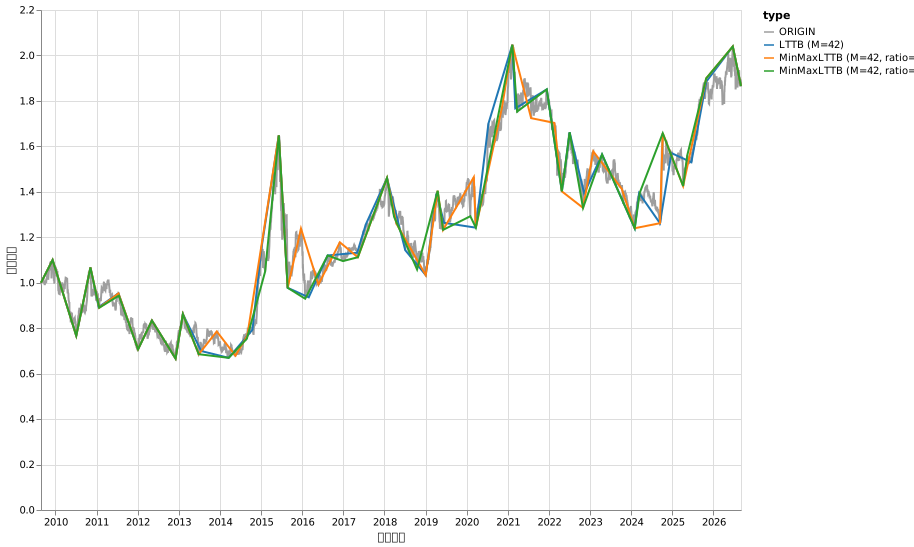
We may draw these conclusions from this diagram.

• Both LTTB and MinMaxLTTB yield similar results, both doing a solid job of preserving the overall visual trend.
• Neither algorithm guarantees that global extremes (peaks and troughs) will be preserved.
• The larger the $ratio$, the closer the MinMaxLTTB output gets to standard LTTB. This makes intuitive sense from the design: a higher $ratio$ means more candidate extreme points are preselected. In the extreme case where every point is preselected, MinMaxLTTB degrades into plain LTTB.